Introduction to the Davinci interface
Contents |
Starting the KRC function
To start the KRC function in davinci, simply run the krc() function:
% davinci
dv> krc()
When started in this manner, the krc function will provide some context and definitions for some of the most common inputs
Simple Runs for Mars
Now let's run KRC for a simple case on Mars to determine the surface temperature in Gale Crater (latitude = -4.5; longitude = 137.4)
dv> out=krc(lat=-4.5,lon=137.5)
Read TEXT file: 61 lines
Found Default File: $DV_SCRIPT_FILES/krc_support/porb_defaults/Mars_Mars.porb.hdf
./Applications/davinci.app/Contents/Resources/library/script_files/krc_support/ti_map2ppd_v4.vicar: VICAR bsq image: 720x360x1, 32 bits
./Applications/davinci.app/Contents/Resources/library/script_files/krc_support/albedo_2ppd.vicar: VICAR bsq image: 720x360x1, 32 bits
./Applications/davinci.app/Contents/Resources/library/script_files/krc_support/mola_2ppd.vicar: VICAR bsq image: 720x360x1, 32 bits

Running KRC model with:

Output:
	Every ~1.000 Ls (1.9083 JD) for 360 seasons starting at 0.10 Ls
	For 96 times per day, every 15 local minutes
	Running model WITH NO temperature prediction
	because DELJUL < 3.0779

For a Surface With:
	29 Layers with uniform material properties and 384 daily model time steps
	and T-dependant material properties
	and an insulating bottom edge condition

With Observation Parameters:
	LATITUDE:  -4.50	LONGITUDE: 137.50
	ELEVATION: -3.606km^	SLOPE/AZIMUTH: 0.00/0.00deg
	ALBEDO: 0.228^		OPACITY: 0.300
	HOUR: All		LS: All

Upper Material:
	INERTIA: 230.00
	CONDUCTIVITY: 0.0502*
	DENSITY: 1770.00*
	SPECIFIC HEAT: 595.55
	POROSITY: 0.40

* = derived value unless overwritten by user
^ = from TES 2ppd map unless overwritten by user
& = ajusted for max authorized value


struct, 14 elements
   tsurf: 96x1x360 array of double, bsq format [276,480 bytes]
   tbol: 96x1x360 array of double, bsq format [276,480 bytes]
   tatm: 96x1x360 array of double, bsq format [276,480 bytes]
   down_ir: 96x1x360 array of double, bsq format [276,480 bytes]
   down_vis: 96x1x360 array of double, bsq format [276,480 bytes]
   time: 96x1x1 array of float, bsq format [384 bytes]
   ls: 1x1x360 array of double, bsq format [2,880 bytes]
   lat: -4.50000
   elev: -3.60558
   layer: struct, 8 elements
       thickness: 28x2x1 array of double, bsq format [448 bytes]
       center: 28x2x1 array of double, bsq format [448 bytes]
       top: 28x2x1 array of double, bsq format [448 bytes]
       center_mass: 28x1x1 array of double, bsq format [224 bytes]
       mass_burden: 28x1x1 array of double, bsq format [224 bytes]
       thermal_scales: 28x1x1 array of double, bsq format [224 bytes]
       tmax: 28x1x360 array of double, bsq format [80,640 bytes]
       tmin: 28x1x360 array of double, bsq format [80,640 bytes]
   anc: struct, 11 elements
       krccom: struct, 5 elements...
       JDate: 1x1x360 array of double, bsq format [2,880 bytes]
       ref_pressure: 1x1x360 array of double, bsq format [2,880 bytes]
       taud: 1x1x360 array of double, bsq format [2,880 bytes]
       total_frost: 1x1x360 array of double, bsq format [2,880 bytes]
       avg_heat_flow: 1x1x360 array of double, bsq format [2,880 bytes]
       frost_alb: 1x1x360 array of double, bsq format [2,880 bytes]
       frost: 1x1x360 array of double, bsq format [2,880 bytes]
       tatm_predict: 1x1x360 array of double, bsq format [2,880 bytes]
       delta_t_rms: 1x1x360 array of double, bsq format [2,880 bytes]
       converge_days: 1x1x360 array of double, bsq format [2,880 bytes]
   version: "v3.2.1"
   alb: 0.228235
   body: "Mars"
The output is a structure containing various model parameters, as well a calculated quantities.
Surface temperatures are stored in .tsurf, local times in .time, and Ls in .ls Local times are stored in the x axis, depth in the y axis (not used yet), and season in the z axis.
So let's plot a diurnal temperature curve at Ls = 0.1 (first ls index):
dv> plot(out.tsurf[,1,1],xaxis=out.time)
dv>
Let's plot a seasonal temperature curve at 0:25 (first time index):
dv> plot(out.tsurf[1,1,],xaxis=out.ls)
dv>
When provided with the coordinates of a specific location on Mars, the krc() function reads some contextual information from external maps:
- the elevation: ELEVATION: -3.606km
- the albedo: ALBEDO : 0.228
Of course, these parameters can be set by the user:
dv> out=krc(lat=-4.5,lon=137.5,ALBEDO=0.22,ELEV=-4.5)
dv>
Frequently, you will want to work with a specific Ls
dv> out=krc(lat=-4.5,lon=137.5,ls=122.45)
dv>
More generally, any parameter listed in an input file can be used as an input; run krc() to see the list of variable names.
dv> out_1=krc(lat=-4.5,lon=137.5,ALBEDO=0.22,ELEV=-4.5,INERTIA=120.,SLOPE=12.,SLOAZI=45.,N24=36,SPEC_HEAT=600.,PTOTAL=610.)
dv> out_2=krc(lat=-4.5,DUSTA=0.91,ARC2=0.6,TAURAT=0.201)
Make sure to read the helplist to familiarize yourself with the definition and range of inputs.
More Advanced Functionalities
In this section, a few more advanced functionality are presented.
- Time-Dependent Albedo
KRC can work with Ls dependent surface albedo values. The input format is a 2 column array, with Ls and albedo values along the y axis.
dv> ALBEDO_ARRAY
dv> 2x12x1 array of float, bsq format [96 bytes]
0.00000	0.230000
30.0000	0.250000
60.0000	0.270000
90.0000	0.250000
120.000	0.230000
150.000	0.220000
180.000	0.220000
210.000	0.250000
240.000	0.230000
270.000	0.250000
300.000	0.270000
330.000	0.250000

dv> out_1=krc(lat=0.,INERTIA=45.,ALBEDO=ALBEDO_ARRAY,hour=4.5)
dv> out_2=krc(lat=0.,INERTIA=45.,ALBEDO=0.24,hour=4.5)
dv> plot(out_1.tsurf,"Variable Albedo",out_2.tsurf,"Fixed Albedo",Xaxis=out_1.ls)
dv>
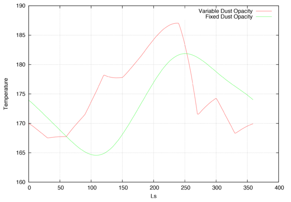
- Time-Dependent Opacity
dv> TAU_ARRAY
2x12x1 array of float, bsq format [96 bytes]
0.00000	0.310000
30.0000	0.320000
60.0000	0.400000
90.0000	0.600000
120.000	0.910000
150.000	0.720000
180.000	0.650000
210.000	0.600000
240.000	0.550000
270.000	0.200000
300.000	0.300000
330.000	0.230000

dv> out_1=krc(lat=0.,INERTIA=45.,TAUD=TAU_ARRAY,hour=4.5)
dv> out_2=krc(lat=0.,INERTIA=45.,TAUD=0.4,hour=4.5)
dv> plot(out_1.tsurf,"Variable Dust Opacity",out_2.tsurf,"Fixed Dust Opacity",Xaxis=out_1.ls)
dv>
- Temperature-dependent Regolith Properties
KRC can work with temperature-dependent thermophysical properties (conductivity and specific heat, but not density). By default, temperature-dependent properties are turned on, but they can be turned off with LkofT="F"
dv> out_1=krc(lat=-4.5,INERTIA=200.,ls=0.,LkofT="T")
dv> out_2=krc(lat=-4.5,INERTIA=200.,ls=0.,LkofT="F")
dv> plot(out_1.tsurf,"I(T)",out_2.tsurf,"Fixed I",Xaxis=out_1.time)
When Temperature dependent properties are allowed (LkofT="T"), KRC expects 4 coefficients describing the conductivity and specific heat:
ConUp0,ConUp1,ConUp2,ConUp3 AND SphUp0,SphUp1,SphUp2,SphUp3
Refer to the helplist to see how these coefficients are used by KRC.
krc() can generate best guess coefficients for ConUp and SphUp based on the thermal inertia provided, assuming basaltic material.
These coefficients are generated by materials_krc(). Make sure to see how this function works to make sure the assumptions are OK for your application.
It is understood that the thermal inertia provided is at 220K (see helplist definitions)
dv> out=krc(lat=0.,INERTIA=700.,ls=356.,Mat1="basalt")
dv> plot(out.tsurf,xaxis=out.time,"Basalt")
dv>
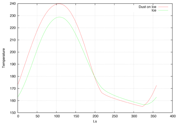
- Two layer Regolith
The interface can handle 2 layers of given thermophysical properties, but the latest version of KRC can be used to define n layers. A future release of the davinci interface will allow to run KRC from davinci with n layers. Be very patient.
To run 2 layers, the user must define:
- the upper and lower inertias (INERTIA, INERTIA2)
- the top material thickness in meters (thick)
evalN1_krc() is the function that links the number of mesh elements in each materials with thick and several numerical stability criteria.
Refer to evalN1_krc() for limits. Large inertia contrasts in conjunction with thin layers is typically not stable.
dv> out_1=krc(INERTIA=50,INERTIA2=2000,thick=5E-4,lat=75.,lon=0.,hour=12.)
dv> out_2=krc(INERTIA=2000,lat=75.,lon=0.,hour=12.)
dv> plot(out_1.tsurf[1,1,],"Dust on Ice",out_2.tsurf[1,1,],"Ice",Xaxis=out_1.ls)
dv>
Simulated One Point Mode
KRC can run a one point mode, usually used to generate lookup tables to derive thermal inertia from a single temperature measurment.
The davinci interface to KRC includes a simulated one point mode, where the user feeds a temperature, and a thermal inertia value is retuned.
THIS SIMULATED MODE IS SIGNIFICANTLY SLOWER THAN THE ORIGINAL KRC ONE POINT MODE
In this mode, the full version of KRC is run for a number of cases (with thermal inertia being the only variable parameter), but an interpolation is used to derive a thermal inertia value.
To run KRC in this mode, amke sure to provide:
- a surface temperature: T
- a local time: hour
- a season: ls
dv> out=krc(lat=0.,lon=0.,T=179.23,hour=2.12,ls=67.)
Found Default File: $DV_SCRIPT_FILES/krc_support/porb_defaults/Mars_Mars.porb.hdf
./Applications/davinci.app/Contents/Resources/library/script_files/krc_support/ti_map2ppd_v4.vicar: VICAR bsq image: 720x360x1, 32 bits
./Applications/davinci.app/Contents/Resources/library/script_files/krc_support/albedo_2ppd.vicar: VICAR bsq image: 720x360x1, 32 bits
./Applications/davinci.app/Contents/Resources/library/script_files/krc_support/mola_2ppd.vicar: VICAR bsq image: 720x360x1, 32 bits

Running KRC model with:

Output:
Every ~8.000 Ls (15.2664 JD) for 45 seasons starting at 0.10 Ls
For 96 times per day, every 15 local minutes
Running model WITH temperature prediction for speed

For a Surface With:
29 Layers with uniform material properties and 384 daily model time steps
and T-dependant material properties
and an insulating bottom edge condition

With Observation Parameters:
       LATITUDE:   0.00	        LONGITUDE:   0.00
       ELEVATION: -1.411km^	SLOPE/AZIMUTH: 0.00/0.00deg
       ALBEDO: 0.186^		OPACITY: 0.300
       HOUR: 2.12		LS: 67.00

Running One-Point Simulation Mode


Interpolating for TI values: 20.00 to 2200.00
       with temperatures: 160.39K to 220.11K
       from table indices: 1 to 40

134.793

dv>
In this example, the surface temperature T=179.23 K at the local time hour=2.12 (02:12AM) and season Ls=67.0 is found to be associated with a thermal inertia of 134.793 Jm-2K-1s-1/2.


