Beginner Tutorial
Contents |
Already Familiar with KRC?
- If you are already familiar with KRC's basic functionality, please see the Advanced Tutorial.
Download KRC or check which Version you have
- To start using KRC, be sure you have already downloaded latest version. If you already have KRC, but do not know if you have the latest version, you can check which version you have here.
Once you have the latest version, it is time to start using KRC.
Getting Started
- To start using KRC, you must first start the Davinci Interface. To learn more about Davinci visit the DavinciWiki
Remember: The KRC Davinci Interface is reffered to as Davinci, and using KRC with input files is referred to as KRC.
Type the following:
$ davinci
dv>
Now, you can start using KRC.
Type the following:
dv> krc()
This command will bring up a the KRC Main Menu:
 This runs the full krc binary mode with the following inputs

IMPORTANT: This interface supports only KRC > v2.3.2

lat       = latitude **Required**
lon       = east longitude (default = 0)
body      = name of the body (Default = "Mars")
bodytype  = kind of body - "planet", "minor", "comet" (Default = "planet")
hour      = hour of day for data to return (default=-32768, all hours)
ls        = ls for data to return (default=-32768, all seasons)
INERTIA   = thermal inertia of upper layers (default from 2ppd TES)
Mat1      = material of upper layers, sets COND, DENSITY, SPEC_HEAT (Default="basalt")
Por1      = porosity of upper layers, affects DENSITY (Default=0.4)
INERTIA2  = thermal inertia of lower layers (Default from 2ppd TES)
Mat2      = material of lower layers, sets COND2, DENS2, SpHeat2 (Default="Mat1")
Por2      = porosity of lower layers, affects DENS2 (Default=Por1)
thick     = top layer thickness (default=0, no layering)
TDEEP     = set bottom layer temperature (default TDEEP=0, IB=0, insulating)
JBARE     = force frost free at specified season (default JBARE=0, no forcing)
SLOPE     = surface slope in degrees (default = 0)
ALBEDO    = albedo (default from lat,lon 2ppd TES)
TAUD      = dust visible opacity (default TAUD= 0.30)
ELEV      = elevation km (default from lat,lon 2ppd MOLA)
SLOAZI    = slope azimuth in degrees east from north (default = 0)
DELLS     = ~delta Ls desired (sets DELJUL automatically, Default = 1)
DELJUL    = delta julian date to increment by (Default = 1.9083)
DJUL      = if LKEY="T", starting Ls (Default = 0.1)
           or start julian date offset from J2000
LKEY      = use Ls DJUL input rather than jullian date (Default ="T")
JDISK     = start "season" to output (Default = 721)
N5        = number of "seasons" to run (Default = 1080)
N24       = number of outputs per day (Default = 96)
LkofT     = use temperature dependant properties (Default = "T")
TPREDICT  = use forward prediction of temperatures for speed (Default ="T")
stability = check for model stability (Default = 0)
outusage  = displays the bin52 file type usage

KRC-ONE like option:
T         = sets a one-point like mode where a TI is returned
           for the specified conditions. This can be an array.

These values are from the standard KRC input file. Defaults from above are
used in place of the master.inp file values.

Enter for more usage
Read TEXT file: 61 lines

Real Value Parameters (Values from default input file)
############################################################################
ALBEDO  = .25       EMISS   = 1.00      INERTIA = 200.0     COND2   = 2.77
DENS2   = 928.0     PERIOD  = 1.0275    SPEC_HEAT= 647.      DENSITY = 1600.
CABR    = 0.11      AMW     = 43.5      ABRPHA  = -0.00     PTOTAL  = 546.0
FANON   = .055      TATM    = 200.      TDEEP   = 180.0     SpHeat2 = 1711.
TAUD    = 0.3       DUSTA   = .90       TAURAT  = 0.5       TWILI   = 0.0
ARC2    = 0.5       ARC3    = -0.00     SLOPE   = 0.0       SLOAZI  = 90.
TFROST  = 146.0     CFROST  = 589944.   AFROST  = .65       FEMIS   = 0.95
AF1     = 0.54      AF2     = 0.0009    FROEXT  = 50.       FD32    = 0.0
RLAY    = 1.2000    FLAY    = .1800     CONVF   = 2.0000    DEPTH   = 0.0
DRSET   = 0.0       DDT     = .0020     GGT     = 0.1       DTMAX   = 0.1
DJUL    = -1222.69  DELJUL  = 17.174822 SOLARDEC= 00.0      DAU     = 1.465
LsubS   = .0        SOLCON  = 1368.     GRAV    = 3.727     AtmCp   = 735.9
ConUp0  = 0.038640  ConUp1  = -0.002145 ConUp2  = 0.002347  ConUp3  = -0.000750
ConLo0  = 2.766722  ConLo1  = -1.298966 ConLo2  = 0.629224  ConLo3  = -0.527291
SphUp0  = 646.6275  SphUp1  = 246.6678  SphUp2  = -49.8216  SphUp3  = 7.9520
SphLo0  = 1710.648  SphLo1  = 721.8740  SphLo2  = 57.44873  SphLo3  = 24.37532

Enter for more
Integer Value Parameters (Values from default input file)
############################################################################
N1      = 20        N2      = 384       N3      = 15        N4      = 19
N5      = 120       N24     = 24        IB      = 0         IC      = 7
NRSET   = 3         NMHA    = 24        NRUN    = 0         JDISK   = 81
IDOWN   = 0         FlxP14  = 45        FlxP15  = 65        KPREF   = 1
K4OUT   = 52        JBARE   = 0         Notif   = 20        IDISK2  = 0
end     = 0

Boolean Parameters (Values from default input file)
############################################################################
LP1     = F         LP2     = T         LP3     = F         LP4     = F
LP5     = F         LP6     = F         LPGLOB  = F         LVFA    = F
LVFT    = F         LkofT   = F         LPORB   = T         LKEY    = F
LSC     = F         spare   = F         LOCAL   = T         Prt76   = F
LPTAVE  = F         Prt78   = F         Prt79   = F         L_ONE   = F

Found Default File: $DV_SCRIPT_FILES/krc_support/porb_defaults/Mars_Mars.porb.hdf
Enter for more
K4OUT = 52.  This interface only supports bin52 output which encapsulates most of the other file formats
NOTE: Recommended parameter changes are listed in the first section.
Please use these paramters with caution. They are meant for advanced users.

N1 (the number of layers, Default=29) is calculated in the function evalN1_krc()
    This function relies on various parameters including FLAY, RLAY, length of the year
    to calculate the minimum number of layers required to reach seasonal skindepth stability
N2 (the number of calculations per day, Default=288) is calculated in the functin evalN2_krc()
    This function relies varous parameters including FLAY, N24, PERIOD

The default model iterates for 2 years before
outputing a full year (N5-JDISK) of data at 1/360th year intervals (DELJUL),
starting at DJUL=0 (in Ls), JDISK=721, DELJUL=1.9083
from 24.0/N24 to 24 by 24.0/N24 (15 minutes with N24=96).

First layer is set at FLAY=0.18 skin depths.
Each successive layer is increased by a factor of RLAY=1.2.

ALBEDO and TAUD can be dynamic if input as
2 x n x 1 arrays. Ls = column 1 and ALBEDO/TAUD = column 2

See the helplist distributed with KRC for variable meanings and default values.

C.Edwards + S.Piqueux 2/13
This menu offers quick guides to the basic input parameters
The next step is to generate simple runs with KRC.
Simple Runs
- Try designating a specific location to run the KRC model.
Use the landing site of the Curiosity Rover within Gale Crater.
Latitude: 4.5o S Longitude: 137.4o E
KRC takes positive values for Northern latitudes and negative values for Southern latitudes. But KRC only takes positive values for longitude. Therefore, Western longitudes must be subtracted from 360o to be input as positive Eastern longitude values.
See the Helplist, Input Parameter Glossary. or use the KRC Main Menu to learn input parameter variable names and definitions.
dv> krc(lat = -4.5, lon = 137.4)
You should see the following output. If you do not see this message, check the previous line and try again.
Found Default File: $DV_SCRIPT_FILES/krc_support/porb_defaults/Mars_Mars.porb.hdf
./nfs/software/davinci_install/share/davinci//library/script_files/krc_support/ti_map2ppd_v4.vicar: VICAR bsq image: 720x360x1, 32 bits
./nfs/software/davinci_install/share/davinci//library/script_files/krc_support/albedo_2ppd.vicar: VICAR bsq image: 720x360x1, 32 bits
./nfs/software/davinci_install/share/davinci//library/script_files/krc_support/mola_2ppd.vicar: VICAR bsq image: 720x360x1, 32 bits

Running KRC model with:

Output:
    Every ~1.000 Ls (1.9083 JD) for 360 seasons starting at 0.10 Ls
    For 96 times per day, every 15 local minutes
    Running model WITH NO temperature prediction
    because DELJUL < 3.0779

For a Surface With:
    29 Layers with uniform material properties and 384 daily model time steps
    and T-dependant material properties
    and an insulating bottom edge condition

With Observation Parameters:
    LATITUDE:  -4.50    LONGITUDE: 137.40
    ELEVATION: -3.606km^    SLOPE/AZIMUTH: 0.00/0.00deg
    ALBEDO: 0.228^        OPACITY: 0.300
    HOUR: All        LS: All

Upper Material:
    INERTIA: 230.00
    CONDUCTIVITY: 0.0502*
    DENSITY: 1770.00*
    SPECIFIC HEAT: 595.55
    POROSITY: 0.40

* = derived value unless overwritten by user
^ = from TES 2ppd map unless overwritten by user
& = ajusted for max authorized value

struct, 14 elements
    tsurf: 96x1x360 array of double, bsq format [276,480 bytes]
    tbol: 96x1x360 array of double, bsq format [276,480 bytes]
    tatm: 96x1x360 array of double, bsq format [276,480 bytes]
    down_ir: 96x1x360 array of double, bsq format [276,480 bytes]
    down_vis: 96x1x360 array of double, bsq format [276,480 bytes]
    time: 96x1x1 array of float, bsq format [384 bytes]
    ls: 1x1x360 array of double, bsq format [2,880 bytes]
    lat: -4.500000000
    elev: -3.605580091
    layer: struct, 8 elements
        thickness: 28x2x1 array of double, bsq format [448 bytes]
        center: 28x2x1 array of double, bsq format [448 bytes]
        top: 28x2x1 array of double, bsq format [448 bytes]
        center_mass: 28x1x1 array of double, bsq format [224 bytes]
        mass_burden: 28x1x1 array of double, bsq format [224 bytes]
        thermal_scales: 28x1x1 array of double, bsq format [224 bytes]
        tmax: 28x1x360 array of double, bsq format [80,640 bytes]
        tmin: 28x1x360 array of double, bsq format [80,640 bytes]
    anc: struct, 11 elements
        krccom: struct, 5 elements...
        JDate: 1x1x360 array of double, bsq format [2,880 bytes]You need not worry about most of this output, as you will most likely not need to investigate the output or script files.
        ref_pressure: 1x1x360 array of double, bsq format [2,880 bytes]
        taud: 1x1x360 array of double, bsq format [2,880 bytes]
        total_frost: 1x1x360 array of double, bsq format [2,880 bytes]
        avg_heat_flow: 1x1x360 array of double, bsq format [2,880 bytes]
        frost_alb: 1x1x360 array of double, bsq format [2,880 bytes]
        frost: 1x1x360 array of double, bsq format [2,880 bytes]
        tatm_predict: 1x1x360 array of double, bsq format [2,880 bytes]
        delta_t_rms: 1x1x360 array of double, bsq format [2,880 bytes]
        converge_days: 1x1x360 array of double, bsq format [2,880 bytes]
    version: "v3.2.1"
    alb: 0.2282352895
    body: "Mars"
Interpreting the Output
You need not worry about the first few lines of output, as you will most likely not need to investigate the output or script files.
The rest of the output is a multi-element structure consisting of model outputs as well as the initial input parameters. Some of these outputs (i.e. Kinetic Surface Temperature, tsurf, Bolometeric Temperature, tbol, and Atmospheric Temperature, tatm, are three dimensional elements where the first dimension contains the values for all hours of a single day, and the third dimension contains all values for all LS of a single year.
If you set the function krc() equal to a variable, you can access the elements contained within the output.
dv> test = krc(lat=12)
To access the elements simply type the variable name followed by a period, then the element you wish to examine. Be careful to keep the dimensions of the element consistent.
To see basic information about the element:
dv> test.tsurf[,,]
96x1x360 array of double, bsq format [276,480 bytes]
Or:
dv> test.tsurf
96x1x360 array of double, bsq format [276,480 bytes]
To see all values for a specific season:
dv> test.tsurf[,,105]
96x1x1 array of double, bsq format [768 bytes]
171.5856935    171.1550320    170.7370510    170.3293537    169.9308028    169.5406723    169.1583461    168.7833589    168.4152575    168.0536924    167.6983010    167.3488043    167.0048976    166.6663525    166.3329117    166.0043847    165.6805461    165.3612358    165.0462598    164.7354822    164.4287279    164.1258806    164.8784105    169.1850639    175.8574576    184.1348010    193.0209648    201.8500108    210.2748614    218.1462596    225.4199940    232.1023999    238.2214758    243.8125454    248.9114546    253.5516366    257.7629989    261.5717402    265.0005054    268.0687358    270.7930092    273.1874139    275.2638321    277.0322298    278.5008521    279.6764380    280.5643349    281.1686471    281.4922865    281.5370772    281.3037515    280.7920112    280.0004782    278.9267210    277.5671609    275.9170552    273.9703619    271.7196781    269.1560659    266.2689434    263.0458944    259.4725498    255.5324779    251.2072449    246.4767807    241.3204027    235.7192896    229.6618763    223.1557308    216.2532801    209.1076064    202.0783448    195.7509294    190.7815122    188.2797335    186.4750573    185.0143727    183.7710532    182.6794830    181.7005257    180.8088599    179.9870621    179.2225887    178.5060773    177.8303253    177.1896796    176.5795809    175.9963471    175.4369088    174.8987397    174.3796661    173.8778849    173.3918072    172.9201071    172.4615814    172.0152291
To see a value for a specific time of day during a specific season:
dv> test.tsurf[13,,105]
167.0048976
More Runs
Now, add some more input parameters into the model. The following line is an example of possible variables that might be included in a simple run.
dv> krc(lat = -4.5, lon = 137.4, ELEV = -4.4, SLOPE = 1.2, SLOAZI = 43)
Elevation is in units of kilometers, slope and azimuth (SLOAZI) are both in degrees. The output should be similar to the previous Run, but with the new specific parameters.
Remember, you can learn more about the KRC parameters in the Helplist, Input Parameter Glossary. or use the KRC Main Menu
Plot model Parameters
Various Example Plots
Here are some examples of plots that KRC can create once the model is understood. View more plots here


Description
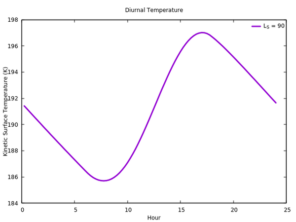
The ability to plot temperature variations with KRC is one of the most useful features with the KRC Davinci Interface. It provides a method to visually inspect surface properties based on changes in time over the course of a single day or an entire year.
We will be plotting the output from the previous run. You must declare this run as a variable in order to plot the output. For example, use KRC_Out.
Example 1: Diurnal Temperature
First, plot Kinetic Surface Temperature as a function of hours for a given season of the year. The seasons are contained in the element "ls". There are 360 values for possible season indicators. Keep in mind ls[1,1,90] is not LS of 90, it is index 90 of ls. LS 90 = ls[1,1,105]
dv> KRC_Out = krc(lat = -4.5, lon = 137.4, ELEV = -4.4, SLOPE = 1.2, SLOAZI = 43)

dv> pplot(KRC_Out.tsurf[,,105], Xaxis = KRC_Out.time, xlabel = "Hour", ylabel = "Kinetic Surface Temperature (K)", plot_title = "Diurnal Temperature", "Daily Temp"]
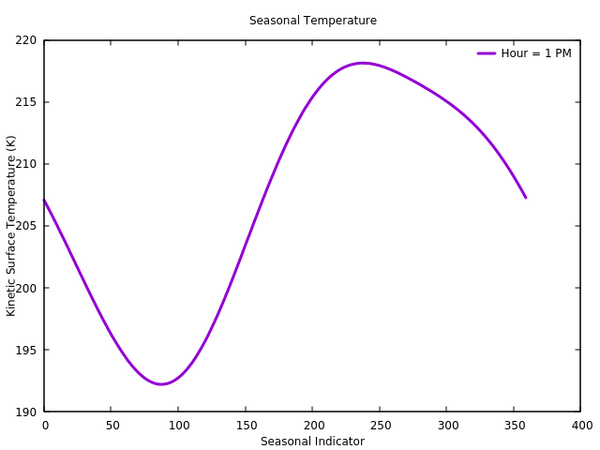
Example 2: Seasonal Temperature
Next, plot Kinetic Surface Temperature as a function of season for a given hour of the day. The given hour of the day is defined by the
dv> pplot(KRC_Out.tsurf[52,,], Xaxis = KRC_Out.ls, xlabel = "Seasonal Indicator", ylabel = "Kinetic Surface Temperature (K)", plot_title = "Seasonal Temperature", "Seasonal Temp")
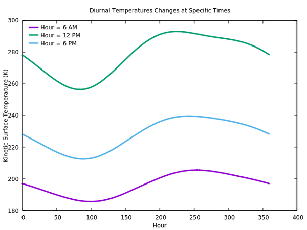
Example 3: Multiple Curves in Same Plot
Now, plot several times of day on the same plot throughout an entire year. Each curve represents a different time of the day. Notice the x-axis range is 0 to 360 (i.e. the full range of LS, or a full year).
dv> pplot({KRC_Out.tsurf[24,,],KRC_Out.tsurf[48,,],KRC_Out.tsurf[72,,]},{"Hour = 6 AM", "Hour = 12 PM", "Hour = 6 PM"}, xaxis = gale.ls, xlabel = "Hour", ylabel = "Kinetic Surface Temperature (K)", plot_title = "Diurnal Temperatures Changes at Specific Times", key = "top left")
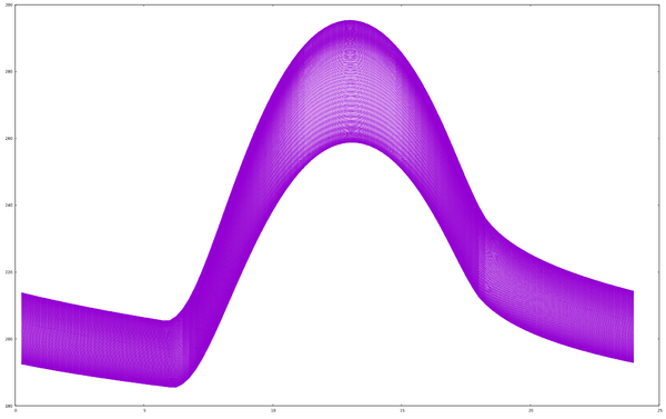
Example 4: Plotting an Entire Season or Day
Now, plot all seasons over an entire day. This will show how daily temperatures change over the course of a year. Each curve will represent a different time of year. Notice the x-axis range is 0 to 24 (i.e. the hours in a day).
dv> pplot(KRC_Out.tsurf[,,], Xaxis = KRC_Out.ls, xlabel = "Seasonal Indicator", ylabel = "Kinetic Surface Temperature (K)", plot_title = " Temperature", "Seasonal Temp")
Knowing What to Plot Based on Analysis' Needs
- The choice on what to plot completely depends on the particular science goals.
Therefore, it is paramount to understand exactly what In order to know what KRC is incredibly flexible and has a wide range of functionality. Therefore, it is important to learn the basic capability of KRC. What can it do? How does it work? How specific can conditions be adjusted within the model? In short, KRC can do a great deal and can vary almost any condition desired. The goal of this wiki page is to introduce new users to KRC and reveal the full capabilities of KRC to both general and more advanced users. Good luck, and happy modeling. Once you fully understand your science goals, and what you hope to prove, determine or represent, you can plot the output.
KRC Modes
Description
There are two modes to use within KRC; Normal and OnePoint. However, OnePoint Mode has an alternative version called Simulated OnePoint Mode.
Normal Mode
- This is the standard mode of operation in Davinci. This takes dozens of possible input parameters to produce the surface temperatures of specific locations on Mars.
OnePoint Mode
NOTE: KRC OnePoint Mode currently does not work. Instead, use Simulated OnePoint Mode
Simulated OnePoint Mode
This mode of operation only applies to davinci and not KRC.
Start davinci as normal.
>davinci
dv>
Now, Simulated OnePoint Mode is used to calculate Thermal Inertias for the surface of Mars.
There are certain required parameters when using Simulated OnePoint Mode:
- lat (as always)
- ls (the seasonal indicator)
- hour (the hour of the day)
- T (a temperature for the surface)
In this case, we will use the standard surface temperature of 220 K, and continue using Gale Crater for the remaining parameters.
dv> krc(lat = -4.5, lon = 137.4, ELEV = -4.4, SLOPE = 1.2, SLOAZI = 43, T = 220, ls = 105, hour = 13)
Found Default File: $DV_SCRIPT_FILES/krc_support/porb_defaults/Mars_Mars.porb.hdf
./nfs/software/davinci_install/share/davinci//library/script_files/krc_support/ti_map2ppd_v4.vicar: VICAR bsq image: 720x360x1, 32 bits
./nfs/software/davinci_install/share/davinci//library/script_files/krc_support/albedo_2ppd.vicar: VICAR bsq image: 720x360x1, 32 bits

Running KRC model with:

Output:
    Every ~8.000 Ls (15.2664 JD) for 45 seasons starting at 0.10 Ls
    For 96 times per day, every 15 local minutes
    Running model WITH temperature prediction for speed

For a Surface With:
    29 Layers with uniform material properties and 384 daily model time steps
    and T-dependant material properties
    and an insulating bottom edge condition

With Observation Parameters:
    LATITUDE:  -4.50    LONGITUDE: 137.40
    ELEVATION: -4.400km^    SLOPE/AZIMUTH: 1.20/43.00deg
    ALBEDO: 0.228^        OPACITY: 0.300
    HOUR: 13.00        LS: 105.00

Running One-Point Simulation Mode


Interpolating for TI values: 2200.00 to 20.00
          with temperatures: 230.53K to 276.58K
         from table indices: 1 to 40

20.00000000


