KRC for Mars
| Line 1: | Line 1: | ||
| − | |||
| − | |||
| − | |||
| − | |||
| − | |||
| − | |||
| − | |||
| − | |||
| − | |||
= Command Line Examples = | = Command Line Examples = | ||
Revision as of 10:04, 16 January 2019
Command Line Examples
KRC is run within Davinci.
> davinci
For Mars, it can be run with as little input as a single latitude, e.g. 25°N:
dv> OUT = krc(lat = 25.)
Model output is saved in structure 'OUT'. The decimal is required for parameters to be initialized as a floating point number. All other model inputs are retrieved from lookup tables (e.g., longitude, surface albedo, thermal inertia etc.).
By default, the output is stored into multidimensional arrays sampled at 96 values per sol and 360 values per Mars year. Hence the structure element surface temperature ('OUT.tsurf') appears as:
tsurf: 96x1x360 array of double, bsq format [276,480 bytes]
Additional fields can be prescribed within the parentheses when calling krc. E.g., the same latitude but for a longitude of 120° and surface albedo of 0.3:
dv> OUT = krc(lat = 25., lon = 120., ALBEDO = 0.3)
If a particular season provided as solar longitude (in units of degrees) is desired, the annual dimension (e.g., 360) is removed. E.g., for Ls = 90° (northern summer solstice):
dv> OUT = krc(lat = 25., ls = 90.)
Now 'OUT.tsurf' has the dimensions of:
tsurf: 96x1x1 array of double, bsq format [768 bytes]
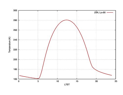
One can plot the diurnal temperature series against local true solar time (LTST) with:
dv> plot(OUT.tsurf , xaxis = OUT.time , "25N, Ls=90" , w = 4 , color = 1)
dv> labelxy("LTST" , "Temperature (K)")
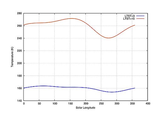
Alternatively, one can prescribe local time and output will be provided for a full Mars year, e.g., for a local time of 3 AM:
dv> OUT = krc(lat = 25., hour = 3.)
'OUT.tsurf' will now be sampled roughly once per degree of solar longitude, e.g.,:
tsurf: 1x1x360 array of double, bsq format [2,880 bytes]
And can be plotted against time (with the addition of 3PM local time as 'OUT_2') with:
dv> plot(OUT.tsurf , xaxis = OUT.ls , "LTST=3" , w = 4 , color = 3,
                 OUT_2.tsurf , xaxis = OUT_2.ls , "LTST=15" , w = 4 , color = 8)
dv> labelxy("Solar Longitude" , "Temperature (K)")
Table of Input Parameters
Other common fields that can be prescribed are included in the table below (*NOTE fields are case sensitive*): [table of parameters (include example ranges?)]
| Parameter | KRC Syntax | Range | Units |
| Latitude | lat | -90–90 | |
| Longitude (°E) | lon | 0–360 | |
| Albedo | ALBEDO | 0–1 | |
| Thermal Inertia | INERTIA | 20–2000 | |
| Elevation | ELEV | ||
| Local True Solar Time | hour | 0–24 | |
| Solar Longitude | ls | 0–360 | |
| Local True Solar Time | hour |
Deriving Thermal Inertia and the "One-Point" Simulation Mode
In order to derive thermal inertia values for a single temperature measurement one can use the simulated one-point mode in KRC. *available only for Mars at present
To use this mode one can call KRC while including the proper spatial and temporal information in addition to a prescribed surface temperature.
For example, if we measured a surface temperature of 190 K at 25°N, 0°W, at Ls = 90° and a local true solar time of 3, we can derive the thermal inertia with:
dv> krc(T = 190., lat = 25., lon = 0., ls = 90., hour = 3.)
Which corresponds to a derived thermal inertia of
284.856
In the above example surface albedo, atmospheric opacity, and elevation was not prescribed. Those values are gathered from lookup tables within KRC, and for this case are equal to:
ELEVATION: -1.942km^
ALBEDO: 0.254^
OPACITY: 0.300
The user can also provide a guess of the thermal inertia, which can speedup the computation, e.g.,:
dv> krc(T = 190., lat = 25., lon = 0., ls = 90., hour = 3., TI_Guess = 200)
Resulting in a derived thermal inertia of
284.941

