Category:KRC Tutorial

Starting the KRC function

To start the KRC function in davinci, simply run the krc() function:

% davinci
dv> krc()

When started in this manner, the krc function will provide some context and definitions for some of the most common inputs

Simple Runs for Mars

Now let's run KRC for a simple case on Mars to determine the surface temperature in Gale Crater (latitude = -4.5; longitude = 137.4)

dv> out=krc(lat=-4.5,lon=137.5)
Read TEXT file: 61 lines
Found Default File: $DV_SCRIPT_FILES/krc_support/porb_defaults/Mars_Mars.porb.hdf
./Applications/davinci.app/Contents/Resources/library/script_files/krc_support/ti_map2ppd_v4.vicar: VICAR bsq image: 720x360x1, 32 bits
./Applications/davinci.app/Contents/Resources/library/script_files/krc_support/albedo_2ppd.vicar: VICAR bsq image: 720x360x1, 32 bits
./Applications/davinci.app/Contents/Resources/library/script_files/krc_support/mola_2ppd.vicar: VICAR bsq image: 720x360x1, 32 bits

Running KRC model with:

Output:
	Every ~1.000 Ls (1.9083 JD) for 360 seasons starting at 0.10 Ls
	For 96 times per day, every 15 local minutes
	Running model WITH NO temperature prediction
	because DELJUL < 3.0779

For a Surface With:
	29 Layers with uniform material properties and 384 daily model time steps
	and T-dependant material properties
	and an insulating bottom edge condition

With Observation Parameters:
	LATITUDE:  -4.50	LONGITUDE: 137.50
	ELEVATION: -3.606km^	SLOPE/AZIMUTH: 0.00/0.00deg
	ALBEDO: 0.228^		OPACITY: 0.300
	HOUR: All		LS: All

Upper Material:
	INERTIA: 230.00
	CONDUCTIVITY: 0.0502*
	DENSITY: 1770.00*
	SPECIFIC HEAT: 595.55
	POROSITY: 0.40

* = derived value unless overwritten by user
^ = from TES 2ppd map unless overwritten by user
& = ajusted for max authorized value 

 
struct, 14 elements
   tsurf: 96x1x360 array of double, bsq format [276,480 bytes]
   tbol: 96x1x360 array of double, bsq format [276,480 bytes]
   tatm: 96x1x360 array of double, bsq format [276,480 bytes]
   down_ir: 96x1x360 array of double, bsq format [276,480 bytes]
   down_vis: 96x1x360 array of double, bsq format [276,480 bytes]
   time: 96x1x1 array of float, bsq format [384 bytes]
   ls: 1x1x360 array of double, bsq format [2,880 bytes]
   lat: -4.50000	
   elev: -3.60558	
   layer: struct, 8 elements
       thickness: 28x2x1 array of double, bsq format [448 bytes]
       center: 28x2x1 array of double, bsq format [448 bytes]
       top: 28x2x1 array of double, bsq format [448 bytes]
       center_mass: 28x1x1 array of double, bsq format [224 bytes]
       mass_burden: 28x1x1 array of double, bsq format [224 bytes]
       thermal_scales: 28x1x1 array of double, bsq format [224 bytes]
       tmax: 28x1x360 array of double, bsq format [80,640 bytes]
       tmin: 28x1x360 array of double, bsq format [80,640 bytes]
   anc: struct, 11 elements
       krccom: struct, 5 elements...
       JDate: 1x1x360 array of double, bsq format [2,880 bytes]
       ref_pressure: 1x1x360 array of double, bsq format [2,880 bytes]
       taud: 1x1x360 array of double, bsq format [2,880 bytes]
       total_frost: 1x1x360 array of double, bsq format [2,880 bytes]
       avg_heat_flow: 1x1x360 array of double, bsq format [2,880 bytes]
       frost_alb: 1x1x360 array of double, bsq format [2,880 bytes]
       frost: 1x1x360 array of double, bsq format [2,880 bytes]
       tatm_predict: 1x1x360 array of double, bsq format [2,880 bytes]
       delta_t_rms: 1x1x360 array of double, bsq format [2,880 bytes]
       converge_days: 1x1x360 array of double, bsq format [2,880 bytes]
   version: "v3.2.1"
   alb: 0.228235	
   body: "Mars"

The output is a structure containing various model parameters, as well a calculated quantities.

Surface temperatures are stored in .tsurf, local times in .time, and Ls in .ls Local times are stored in the x axis, depth in the y axis (not used yet), and season in the z axis.

So let's plot a diurnal temperature curve at Ls = 0.1 (first ls index):

dv> plot(out.tsurf[,1,1],xaxis=out.time)
dv>  

Let's plot a seasonal temperature curve at 0:25 (first time index):

dv> plot(out.tsurf[1,1,],xaxis=out.ls)
dv>

When provided with the coordinates of a specific location on Mars, the krc() function reads some contextual information from external maps:

- the elevation: ELEVATION: -3.606km

- the albedo: ALBEDO : 0.228

Of course, these parameters can be set by the user:

dv> out=krc(lat=-4.5,lon=137.5,ALBEDO=0.22,ELEV=-4.5)
dv> 

Frequently, you will want to work with a specific Ls

dv> out=krc(lat=-4.5,lon=137.5,ls=122.45)
dv>

More generally, any parameter listed in an input file can be used as an input; run krc() to see the list of variable names.

dv> out_1=krc(lat=-4.5,lon=137.5,ALBEDO=0.22,ELEV=-4.5,INERTIA=120.,SLOPE=12.,SLOAZI=45.,N24=36,SPEC_HEAT=600.,PTOTAL=610.)
dv> out_2=krc(lat=-4.5,DUSTA=0.91,ARC2=0.6,TAURAT=0.201)

Make sure to read the helplist to familiarize yourself with the definition and range of inputs.

More Advanced Functionalities

In this section, a few more advanced functionality are presented.

• Time-Dependent Albedo

KRC can work with Ls dependent surface albedo values. The input format is a 2 column array, with Ls and albedo values along the y axis.

dv> ALBEDO_ARRAY
dv> 2x12x1 array of float, bsq format [96 bytes]
0.00000	0.230000	
30.0000	0.250000	
60.0000	0.270000	
90.0000	0.250000	
120.000	0.230000	
150.000	0.220000	
180.000	0.220000	
210.000	0.250000	
240.000	0.230000	
270.000	0.250000	
300.000	0.270000	
330.000	0.250000
 
dv> out_1=krc(lat=0.,INERTIA=45.,ALBEDO=ALBEDO_ARRAY,hour=4.5)
dv> out_2=krc(lat=0.,INERTIA=45.,ALBEDO=0.24,hour=4.5)
dv> plot(out_1.tsurf,"Variable Albedo",out_2.tsurf,"Fixed Albedo",Xaxis=out_1.ls)
dv>

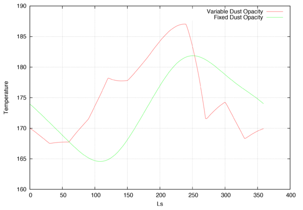
• Time-Dependent Opacity

dv> TAU_ARRAY

2x12x1 array of float, bsq format [96 bytes]
0.00000	0.310000	
30.0000	0.320000	
60.0000	0.400000	
90.0000	0.600000	
120.000	0.910000	
150.000	0.720000	
180.000	0.650000	
210.000	0.600000	
240.000	0.550000	
270.000	0.200000	
300.000	0.300000	
330.000	0.230000	
 
dv> out_1=krc(lat=0.,INERTIA=45.,TAUD=TAU_ARRAY,hour=4.5)
dv> out_2=krc(lat=0.,INERTIA=45.,TAUD=0.4,hour=4.5)
dv> plot(out_1.tsurf,"Variable Dust Opacity",out_2.tsurf,"Fixed Dust Opacity",Xaxis=out_1.ls)
dv>

• Temperature-dependent Specific heat

• Temperature-dependent Conductivity

• Two layer Regolith